A Similarity Graph of Distances

Brian Muchmore

2026-07-14

“To understand is to perceive patterns.”

-Isaiah Berlin, The proper study of mankind, p 129

The metric as the object of study

Most analyses combine many things — data sources, features, whole OMICs. But combining patterns before each one has its own pattern sorted out is garbage-in-garbage-out. This vignette turns the lens around: at the level of a single dataset, where each view is a distance metric, which distances should be combined?

The idea is to build many distances, measure how much they agree, and treat that agreement as its own relatedness matrix — a similarity graph of distances. Strongly agreeing metrics are partly redundant; weakly agreeing ones each add information. That is what tells you what to fuse.

set.seed(1)
idx <- c(1:5, 61:65, 121:125)
cell_cycle <- as.matrix(data_cell_cycle[idx, -1])[, 1:50]
storage.mode(cell_cycle) <- "double"
rownames(cell_cycle) <- paste0(substr(data_cell_cycle$Cell_cycle[idx], 1, 2), "_", idx)

Build several distances

d <- precise_dist(cell_cycle,
                  dists = c("euclidean", "manhattan", "canberra", "minkowski_1.5"),
                  verbose = FALSE)
d[, c("distance", "type")]
#> # A tibble: 4 × 2
#>   distance      type    
#>   <chr>         <chr>   
#> 1 euclidean     distance
#> 2 manhattan     distance
#> 3 canberra      distance
#> 4 minkowski_1.5 distance

Measure agreement

precise_correlations() runs a Mantel test between every pair of matrices and returns a statistic (correlation) matrix and a signif matrix. It requires a single, coherent type — coerce first with precise_transform() if needed.

d <- precise_transform(d, to = "distance")
agree <- precise_correlations(d, method = "pearson", permutations = 99,
                              verbose = FALSE)
round(agree$statistic, 2)
#>               euclidean manhattan canberra minkowski_1.5
#> euclidean          1.00      0.97     0.41          0.99
#> manhattan          0.97      1.00     0.42          0.99
#> canberra           0.41      0.42     1.00          0.42
#> minkowski_1.5      0.99      0.99     0.42          1.00

See the agreement

The agreement view of precise_viz() renders that matrix as two panels — the statistic and its significance — sharing one clustered ordering, so redundant blocks of metrics line up visually.

ag <- precise_viz(d, views = "agreement",
                  agreement = agree,
                  verbose = FALSE)
ag$panel[[1]]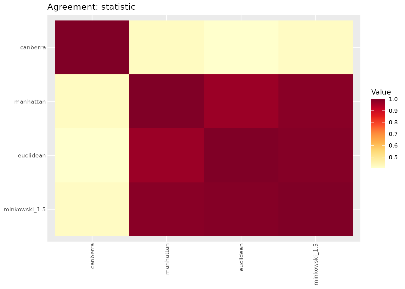

If you prefer an interactive heatmap, the suggested heatmaply package renders the same matrix directly:

heatmaply::heatmaply(agree$statistic)

Act on it: fuse the chosen distances

Having seen which metrics agree, fuse them into a consensus. precise_fusion() takes the whole typed collection and returns one matrix per method.

f <- precise_fusion(d, methods = "mean", verbose = FALSE)
f[, c("method", "type")]
#> # A tibble: 1 × 2
#>   method type    
#>   <chr>  <chr>   
#> 1 mean   distance

The consensus is itself a typed matrix, ready for precise_graph() and precise_viz() — the metric-selection question answered by looking, not assuming.