All Available Views

Brian Muchmore

2026-07-14

“What is to be sought in designs for the display of information is the clear portrayal of complexity. Not the complication of the simple; rather the task of the designer is to give visual access to the subtle and the difficult - that is, the revelation of the complex.”

-Edward Tufte

The typed visualization router

precise_viz() is a single router over the typed outputs of the other tiers. You name the views you want; it returns a tibble with one row per input matrix per view, each panel a ready-to-print ggplot object by default. Plotly is available as an optional renderer through per-view engine = "plotly" parameters. The router is pure: it never builds new relatedness matrices, never fuses, and never infers a matrix’s type from its values — it only computes the visualization data a view declares (a dendrogram order, layout coordinates, an embedding, an agreement matrix).

set.seed(1)
idx <- c(1:5, 61:65, 121:125)
cell_cycle <- as.matrix(data_cell_cycle[idx, -1])[, 1:50]
storage.mode(cell_cycle) <- "double"
rownames(cell_cycle) <- paste0(substr(data_cell_cycle$Cell_cycle[idx], 1, 2), "_", idx)
cell_cycle_groups <- setNames(data_cell_cycle$Cell_cycle[idx], rownames(cell_cycle))

d <- precise_dist(cell_cycle, dists = c("euclidean", "manhattan", "canberra"),
                  verbose = FALSE)
g <- precise_graph(d, methods = "knn", params = list(knn = list(k = 3)),
                   verbose = FALSE)

Each view accepts a particular input type (heatmap takes either; embedding needs a distance; graph_layout needs a similarity/adjacency; agreement is a collection view). Requesting an incompatible view errors rather than silently converting.

heatmap — both types

A tile map with type-aware hierarchical ordering (cluster = TRUE by default; method is passed to hclust unaltered). cluster = FALSE browses the matrix in input order.

precise_viz(
  d,
  views = "heatmap",
  params = list(heatmap = list(engine = "ggplot2")),
  verbose = FALSE
)$panel[[1]]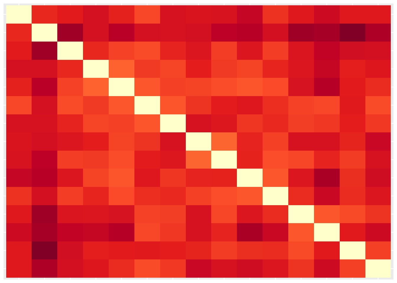

embedding — distance input

Two-dimensional coordinates rendered with ggplot2. The default method = "umap" uses uwot; method = "mds" is the explicit dependency-free fallback, and method = "tsne" is available when Rtsne is installed. A color vector can be named by observation so the annotation remains correct even if rows are reordered upstream. UMAP exposes the controls that usually change the shape of the display: n_neighbors, min_dist, and spread. t-SNE is explicit about its own controls: perplexity, theta, max_iter, eta, and exaggeration_factor are passed through to Rtsne.

precise_viz(
  d,
  views = "embedding",
  params = list(
    embedding = list(
      method = "umap",
      n_neighbors = 10,
      min_dist = 0.01,
      spread = 1,
      engine = "ggplot2",
      seed = 42,
      color = cell_cycle_groups,
      show_labels = FALSE
    )
  ),
  verbose = FALSE
)$panel[[1]]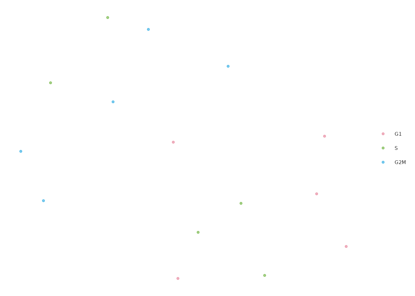

The same view can produce a Plotly widget when interactive hover and zoom are useful. The matrix and coordinates are the same kind of artifact; only the renderer changes.

precise_viz(
  d[1, ],
  views = "embedding",
  params = list(
    embedding = list(
      method = "umap",
      n_neighbors = 10,
      min_dist = 0.01,
      spread = 1,
      engine = "plotly",
      seed = 42,
      color = cell_cycle_groups,
      show_labels = FALSE
    )
  ),
  verbose = FALSE
)$panel[[1]]

Three-dimensional embeddings are explicit. ggplot2 remains the default 2-D renderer; use Plotly or threejs when the extra dimension is part of the visual question.

precise_viz(
  d[1, ],
  views = "embedding",
  params = list(
    embedding = list(
      method = "mds",
      dimensions = 3,
      engine = "threejs",
      seed = 42,
      color = cell_cycle_groups,
      show_labels = FALSE,
      size = 1
    )
  ),
  verbose = FALSE
)$panel[[1]]

precise_viz(
  d[1, ],
  views = "embedding",
  params = list(
    embedding = list(
      method = "tsne",
      dimensions = 3,
      engine = "plotly",
      seed = 42,
      perplexity = 4,
      theta = 0.5,
      max_iter = 1000,
      eta = 200,
      exaggeration_factor = 12,
      color = cell_cycle_groups,
      show_labels = FALSE
    )
  ),
  verbose = FALSE
)$panel[[1]]

graph_layout — similarity/adjacency input

An igraph layout of a graph matrix — precise_graph() output is the primary citizen. layout = "mds" (default) and "kk" are deterministic; "fr" uses the seed.

precise_viz(
  g,
  views = "graph_layout",
  params = list(
    graph_layout = list(
      engine = "ggplot2",
      color = cell_cycle_groups,
      show_labels = FALSE
    )
  ),
  verbose = FALSE
)$panel[[1]]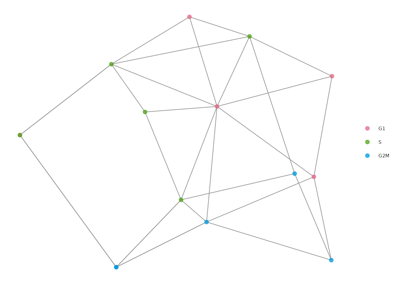

precise_viz(
  g[1, ],
  views = "graph_layout",
  params = list(
    graph_layout = list(
      engine = "plotly",
      color = cell_cycle_groups,
      show_labels = FALSE
    )
  ),
  verbose = FALSE
)$panel[[1]]

The same graph view can be rendered as a 3-D graph or as a 3-D scatter of the vertex layout. The graph render keeps edges; the scatter render suppresses edges when the object-level arrangement is easier to inspect without them.

precise_viz(
  g[1, ],
  views = "graph_layout",
  params = list(
    graph_layout = list(
      layout = "fr",
      dimensions = 3,
      engine = "threejs",
      render = "graph",
      seed = 42,
      color = cell_cycle_groups,
      show_labels = FALSE,
      size = 1
    )
  ),
  verbose = FALSE
)$panel[[1]]

precise_viz(
  g[1, ],
  views = "graph_layout",
  params = list(
    graph_layout = list(
      layout = "fr",
      dimensions = 3,
      engine = "threejs",
      render = "scatter",
      seed = 42,
      color = cell_cycle_groups,
      show_labels = FALSE,
      size = 1
    )
  ),
  verbose = FALSE
)$panel[[1]]

An interactive visNetwork widget is available when that suggested package is installed:

precise_viz(g, views = "graph_layout",
            params = list(graph_layout = list(interactive = TRUE)))$panel[[1]]

agreement — a collection view

Render a precomputed precise_correlations() result as two rows — a statistic heatmap and a significance heatmap — sharing one clustered metric order.

agreement <- precise_correlations(
  d,
  method = "pearson",
  permutations = 99,
  seed = 1,
  verbose = FALSE
)
ag <- precise_viz(d, views = "agreement",
                  params = list(agreement = list(engine = "ggplot2")),
                  agreement = agreement,
                  verbose = FALSE)
ag$panel_id
#> [1] "agreement__statistic"    "agreement__significance"
ag$panel[[1]]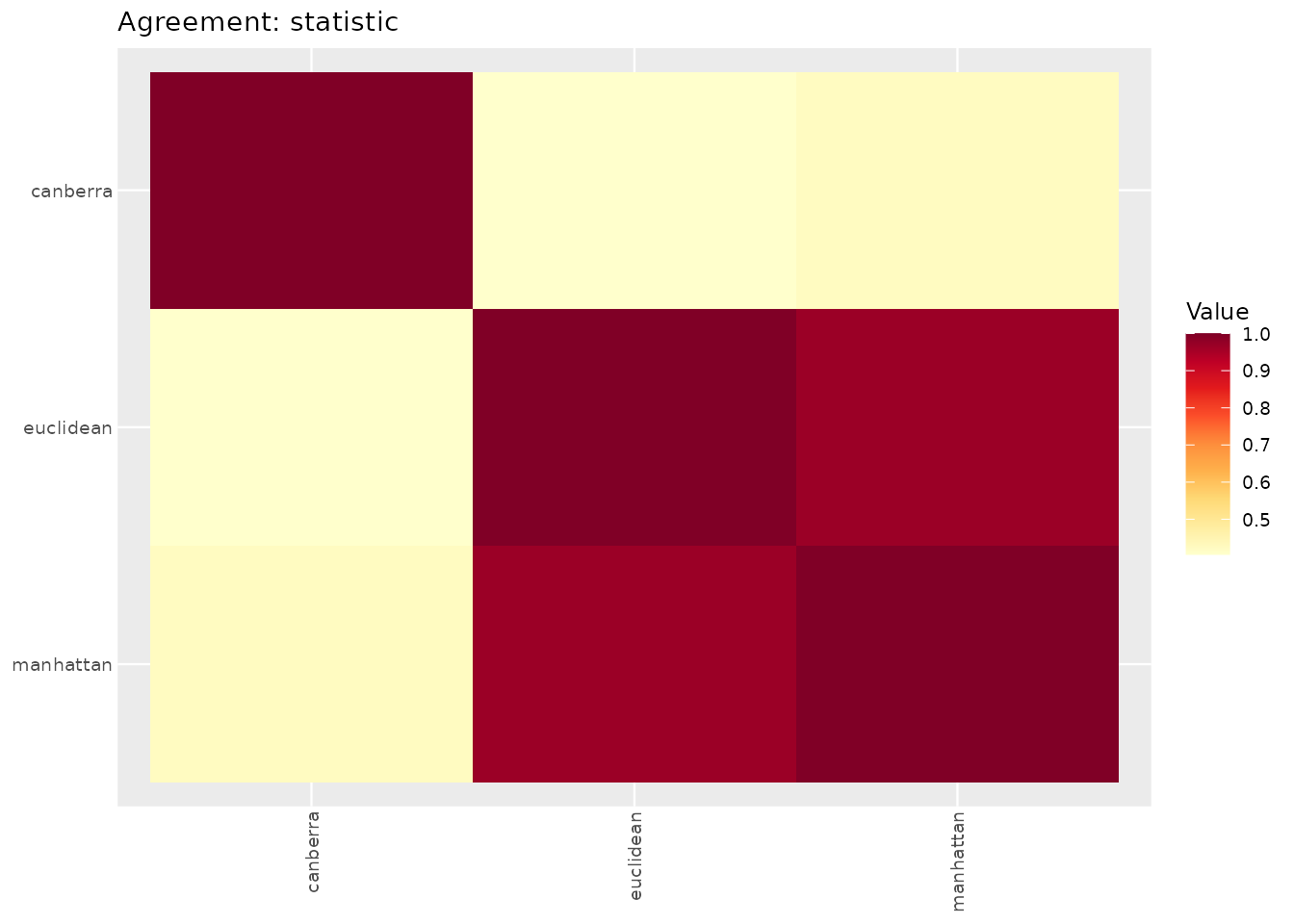

Browsing many panels

Request several views at once and every panel lands in one tibble; the suggested trelliscopejs package can browse them interactively via precise_trellis():

panels <- precise_viz(d, views = c("heatmap", "embedding"), verbose = FALSE)
precise_trellis(panels)